Data-Driven Domain of Shapes

Input to define domain:

• Dataset of 2D shapes (cross sections) with consistent landmarks both in number and reparametrization—i.e., each discrete shape is represented by the same number of landmarks generated by a consistent CST-cosine reparametrization over the shape

• Dependencies detailed below

import os
import numpy as np
# G2Aero
from g2aero.PGA import Grassmann_PGAspace, SPD_TangentSpace
from g2aero.manifolds import ProductManifold, Dataset
from g2aero import SPD as spd
from g2aero import Grassmann as gr

#Plotting
import pandas as pd
import seaborn as sns
import matplotlib.pyplot as plt
%matplotlib inline

Read airfoil data from subdirectory

We begin by loading a saved data set of consistently reparametrized discrete airfoil shapes stored in one of the .npz files in data/airfoils/. This specific set of airfoils represent 1,000 perturbations of \(13\) baseline airfoils from the NREL 5MW and IEA 15MW reference wind turbines. Baseline airfoils are defined by a nominal set of \(18\) CST coefficients (including \(2\) coefficients corresponding to the trailing edge thickness). We then perturb these \(18\) coefficients by up to \(20\%\) of their original value to create the data set.

shapes_folder  = os.path.join(os.getcwd(), '../../data/airfoils/', )
# this is a nice set of randomly generated CST shapes for wind turbine design provided by Andrew Glaws
shapes = np.load(os.path.join(shapes_folder, 'CST_shapes_TE_gap.npz'))['shapes']
print("Dataset:")
print(f"Shape of data = {shapes.shape}")
print(f"N_shapes = {shapes.shape[0]}")
print(f"n_landmarks in every shape = {shapes.shape[1]}")

Dataset:
Shape of data = (13000, 401, 2)
N_shapes = 13000
n_landmarks in every shape = 401

Two types of Landmark-Affine standartization

To map existing airfoil shapes to the elements of Grassmann manifold we using landmark-affine (LA) standardization. There are two types of LA standardization implemented:

• the singular value decomposition (SVD);

• the related polar decomposition.

Note that our implementation utilizes the polar decomposition by default, except when we work with blade interpolation that utilizes the routine GrassmannInterpolator to Procrustes match ordered cross sections to mitigate large variations in the splines of affine deformations.

#landmark-affine (LA) standardization using SVD
shapes_gr1, M, b = gr.landmark_affine_transform(shapes)
#landmark-affine (LA) standardization using polar decomposition
shapes_gr2, P, b = spd.polar_decomposition(shapes)

Build PGA space and get coordinates

Next, we build the Grassmann PGA space from the data set of airfoil shapes. The Grassmann_PGAspace.create_from_dataset() method returns a gr_pga object and an array of normal coordinates T spanning a subspace at the tangent space of the Karcher mean defining a section through the Grassmannian.

# compute Karcher mean and run PGA to define coordinates
from time import time
t1 = time()
gr_pga, T = Grassmann_PGAspace.create_from_dataset(shapes)
t2 = time()
print(t2-t1)

SPD manifold
Karcher mean convergence:
||V||_F = 0.40098078989714303
||V||_F = 6.627185577611687e-05
||V||_F = 2.7465446045536334e-07
||V||_F = 1.967192062945062e-09
Grassmann manifold
Karcher mean convergence:
||V||_F = 0.10235806971182138
||V||_F = 0.00015526889897758003
||V||_F = 2.7114758181406616e-07
||V||_F = 5.985411586299064e-10
31.990497827529907

Similarly, we can separately compute an intrinsic mean and define normal coordinates over the symmetric positive definite (SPD) matrices.

# We can do it manually if already provided matrices `P`
P0 = spd.Karcher(P)
L3, S3, ell = spd.PGA(P0, P)

SPD manifold
Karcher mean convergence:
||V||_F = 0.40098078989714303
||V||_F = 6.627185577611687e-05
||V||_F = 2.7465446045536334e-07
||V||_F = 1.967192062945062e-09

The set of all \(2\)-by-\(2\) SPD matrices is three dimensional. Generally, we utilize the full dimensionality of this space. In the specific case of airfoils, only \(2\) dimensions may be requried to fixed chordal (horizontal) scaling. Consequently, we omit the eigendecomposition of PGA and simply work with the full set of normal coorinates returned by SPD_TangentSpace.create_from_dataset(). The method returns the spd_tan object and an array of normal coordinates T_spd spanning a subspace at the tangent space of the SPD Karcher mean.

spd_tan, T_spd = SPD_TangentSpace.create_from_dataset(shapes)

SPD manifold
Karcher mean convergence:
||V||_F = 0.40098078989714303
||V||_F = 6.627185577611687e-05
||V||_F = 2.7465446045536334e-07
||V||_F = 1.967192062945062e-09
Grassmann manifold
Karcher mean convergence:
||V||_F = 0.10235806971182138
||V||_F = 0.00015526889897758003
||V||_F = 2.7114758181406616e-07
||V||_F = 5.985411586299064e-10

Alternatively, we can automate the construction of the product submanifold using standardized shapes as elements of Grassmann manifold and rescaling matrices as elements of SPD manifold as data. The resulting product_manifold object contains product_manifold.gr_pga_space equivalent to the gr_pga object built above and product_manifold.spd_tan_space equivalent to the spd_tan object built above.

product_manifold = ProductManifold(shapes)
gr_pga = product_manifold.gr_pga_space
T = gr_pga.t

Grassmann manifold
Karcher mean convergence:
||V||_F = 0.10235806971182138
||V||_F = 0.00015526889897758003
||V||_F = 2.7114758181406616e-07
||V||_F = 5.985411586299064e-10
SPD manifold
Karcher mean convergence:
||V||_F = 0.40098078989714303
||V||_F = 6.627185577611687e-05
||V||_F = 2.7465446045536334e-07
||V||_F = 1.967192062945062e-09

Grassmann manifold PGA
SPD manifold Tangent space

Next, we visualize the decay in eigenvalues of the sample covariance of normal coordinates to infer a maximum dimensionality of the submanifold.

# visualize the decay in the first 40 Grassmann eigenvalues (SPD is three dimensional)
fig, ax = plt.subplots(1, 1)
plt.stem(gr_pga.S[:41]**2)
plt.yscale('log')
plt.grid(True, which='both')
plt.xlabel('eigenvalue index')
plt.ylabel('eigenvalue')

Text(0, 0.5, 'eigenvalue')

Evidently, this space is only 18 dimensional. This is consistent with the dimension of the CST expansions used to generate the data. (according to the researchers responsible for carefully currating this database of wind turbine shapes) Now that we have computed the necessary approximation of intrinsic statistical moments, basis for the tangent space, and normal coordinates let’s save them so we don’t have to repeat these computations.

# save the computed Grassmannian PGA space
gr_pga.save_to_file(os.path.join(shapes_folder,'../pga_space/', 'CST_Gr_PGA.npz'))
# also save the SPD PGA space and SPD tangent space
np.savez(os.path.join(shapes_folder,'../pga_space/', 'CST_SPD_PGA.npz'),
         data=P, karcher_mean=P0, basis=L3, coords=ell, weights=S3)
spd_tan.save_to_file(os.path.join(shapes_folder,'../pga_space/', 'CST_SPD_Tangent.npz'))

To visualize this Grassmann PGA space, we plot the first four out of 2*(n_landmarks - 2) ordered normal coordinates over the Grassmannian as scatterplots and marginal pdfs on the first plot. The second plot visualize the SPD normal coordinates.

coord_names = ['$t_1$', '$t_2$', '$t_3$', '$t_4$']
df_all = pd.DataFrame(data=T[:, :4], columns=coord_names)
sns_plot = sns.pairplot(df_all, x_vars=coord_names, y_vars=coord_names,
                        diag_kind='kde', corner=True, plot_kws=dict(s=15))

coord_names = ['$s_1$', '$s_2$', '$s_3$']
df_all = pd.DataFrame(data=T_spd, columns=coord_names)
sns_plot = sns.pairplot(df_all, x_vars=coord_names, y_vars=coord_names,
                        diag_kind='kde', corner=True, plot_kws=dict(s=15))

Low-dimensional shape reconstruction

Let’s try reconstructing a shape using fewer normal coordinates over the Grassmann (low-dimensional PGA space) and compare it to the original shape. Here we set the reduced number of parameters (the dimension of PGA space) to r=4 and choose the shape with index j=1 for demonstration. We also need to calculate LA standardization. LA standardized shapes and corresponding affine transformation is stored in the data object of Dataset class.

# assign r as the dimension of the PGA shape
r = 4 # should always be less than or equal to 2*(n_landmarks - 2)
# pick a shape based on index from the dataset
j = 1 # should be less than or equal to N_shapes-1
# save LA standardized shapes and corresponding affine transformation
data = Dataset(shapes)

First, we demonstrate that this is a distinct element of the Grassmannian. Using the Grassmannian distance (square root of the sum of squared principal anlges between representative shape elements), we emphasize that we are moving along a different (reduced dimension) section of the Grassmannian given a non-zero Grassmannian distance.

# transform from PGA space to element on Grassmann
shape_gr_new = gr_pga.PGA2gr_shape(T[j,:r], original_shape_gr=data.shapes_gr[j])
# compute Grassmannian distance error
err_gr = gr.distance(shape_gr_new, data.shapes_gr[j])
print(f'Grassmannian distance: {err_gr}')

Grassmannian distance: 0.03607142623675289

Then, we compute a worst-case Euclidean error (maximum over Euclidean distances between row-wise pairs of shape landmarks) to offer a human interpretable notion of error in the reconstructed image of the shape in the plane. This reconstruction utilizes a consistent right inverse with nominal M[j] and b[j] defined by the LA standardization of the original shape.

def norm_inf2(sh1, sh2):
    d = np.max(np.linalg.norm(sh1-sh2, ord=2, axis=1))
    return d

# transform from PGA space to physical scales
phys_shape = gr_pga.PGA2shape(T[j,:r], M=data.M[j], b=data.b[j],
                           original_shape_gr=data.shapes_gr[j])
# compute worst-case Euclidean error in row-wise landmarks
err_inf2 = norm_inf2(phys_shape, shapes[j])
print(f'Worst-case Euclidean error: {err_inf2}')

Worst-case Euclidean error: 0.004075096848161961

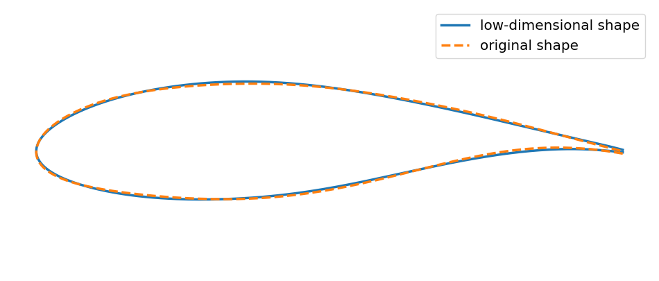
With only four dimensions, the error in the reconstruction of this particular example shape is quite small. Finally, we overlay the low-dimensional shape with the original shape to visualze the magnitude of the mis-match over physically relevant scales.

fig, ax = plt.subplots(1, 1, figsize=(12, 5))
plt.plot(phys_shape[:, 0], phys_shape[:, 1], lw=2.5, label='low-dimensional shape')
plt.plot(shapes[j, :, 0], shapes[j, :, 1], '--', lw=2.5, label='original shape')
plt.axis('off')
ax.axis('equal')
ax.legend(fontsize='x-large')

<matplotlib.legend.Legend at 0x7fd691535460>